In the least square method, the regression model is established in such a way that
"The sum of the squares of the vertical distances of different points (residuals) from the regression line is minimized"
When the relationship between the variables is not linear (one has a non-linear regression model), one may
- try to transform the data to linearize the relationship,
- fit polynomial or complex spline model to the data, or
- fit a non-linear regression to the data.
In the non-linear regression model, a function is specified by a set of parameters to fit the data. The non-linear least squares approach is used to estimate such parameters. In R, the nls() is used to approximate the non-linear function using a linear one and iteratively try to find the best parameter values.
Some frequently used non-linear regression models are listed in the Table below.
| sr no. | Name | Model |
|---|---|---|
| 1) | Michaelis-Menten | $y=\frac{ax}{1+bx}$ |
| 2) | Two-parameter asymptotic exponential | $y=a(1-e^{-bx})$ |
| 3) | Three-parameter asymptotic exponential | $y=a-be^{-cx}$ |
| 4) | Two parameter Logistic | $y=\frac{e^{a+bx}}{1+e^{a+bx}}$ |
| 5) | Three parameter Logistic | $y=\frac{a}{1+be^{-ex}}$ |
| 6) | Weibull | $y=a-be^{-cx^d}$ |
| 7) | Gompertz | $y=e^{-be^{-cx}}$ |
| 8) | Ricker curves | $y=axe^{-bx}$ |
| 9) | Bell-Shaped | $y=a \, exp(-|bx|^2)$ |
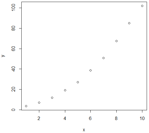
Let’s fit the Michaelis-Menten non-linear function to the data given below.
x <- seq(1, 10, 1)
y <- c(3.7, 7.1, 11.9, 19, 27, 38.5, 51, 67.7, 85, 102)

nls_model <- nls(y ~ a * x/(1 + b * x), start = list(a = 1, b = 1))

summary(nls_model)
The output of the above code for the Michaelis-Menten non-linear function is
#### Output
Formula: y ~ a * x/(1 + b * x)

Parameters:
   Estimate Std. Error t value Pr(>|t|)
a  4.107257   0.226711   18.12 8.85e-08 ***
b -0.060900   0.002708  -22.49 1.62e-08 ***
---
Signif. codes:  0 ‘***’ 0.001 ‘**’ 0.01 ‘*’ 0.05 ‘.’ 0.1 ‘ ’ 1

Residual standard error: 2.805 on 8 degrees of freedom

Number of iterations to convergence: 11
Achieved convergence tolerance: 6.354e-06
Let us plot the non-linear predicted values from 10 data points of newly generated x-values
new.data <- data.frame(x = seq(min(x), max(x), len = 10))

plot(x, y)
lines(new.data$x, predict(nls_model, newdata = new.data) )
The sum of squared residuals and the confidence interval of the chosen values of the coefficient can be obtained by issuing the commands,
sum(resid(nls_model)^2)
# or
print(sum(resid(nls_model)^2))
confint(nls_model)
# or
print(confint(nls_model))
Note that the formula for nls() does not use special coding in linear terms, factors, interactions, etc. The right-hand side in the expression nls() computes the expected value to the left-hand side. The start argument contains the list of starting values of the parameter used in the expression and is varied by the algorithm.